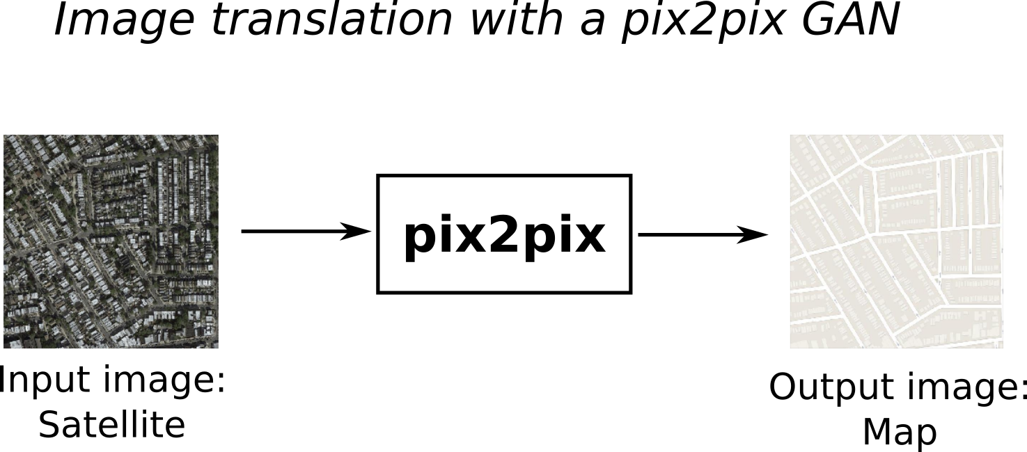
Image-to-image translation with a pix2pix GAN and Keras¶

Back to index

Automatic image-to-image translation is defined (in the pix2pix paper) as the task of translating a representation of a scene (image) into a different representation, given sufficient training data. Such a task for example can be translating a grayscale image into its colorized version. The pix2pix method introduces a conditional deep convolutional generative adversarial network (GAN) for this task. If the reader is not familiar with some of the previous keywords, here are some resources to quickly catch-up on GANs:

The basic idea is that the network consists of two parts: the generator $G$ and the discriminator $D$. The generator tries to generate as realistic images as possible for the task at hand, while the discriminator is basically a binary classifier that tries to separate fake (generated) images from true images of the training set. As the network trains, both $G$ and $D$ become incremetally better at their respective competing roles. After training, the generator is capable of producing as realistic images as possible, in this case corresponding to translations of the input image.

Note: Image translation refers to shifting an image by a number of pixels in the x and/or y axes and should not be confused with the concept of image-to-image translation introduced above.

In this tutorial, we will implement the pix2pix model in keras and use it to predict the map representation of a satellite image. The same concept is visualized in the figure below:

concept

Dataset¶

We will use the Maps dataset, also used in the pix2pix original publication. A download link can be found here. Decompressing the archive results into two folders: "training" (1096 images) and "validation" (1098 images). We will use the training folder for training the pix2pix model and will split the data of the validation folder into separate validation and test sets of $\frac{1098}{2} = 449$ images each. In general, a validation set is not useful for GANs, but we will put that to the test. Each image corresponds to 1200x600 pixels and includes both satellite and map modes side-by-side. As part of pre-processing we will split each image in half, resulting into two 600x600 images and subsequently resize each image to 256x256 pixels to fit the dimensions of the pix2pix model. Last, we will normalize each image so that its pixel values lie in the $[-1,+1]$ range, as suggested for GANs.

Training a GAN¶

Training a GAN is trickier than training a conventional neural network since it requires maintaining a balance between the generator and the discriminator during the training process. If one of the two strongly overpowers the other, the training will fail. Additionally, validation data is not useful and as such, neither is monitoring the validation loss to assess overfitting and/or implement early stopping. Last, training stable GANs requires a number of architectural decisions that are counter intuitive compared to "standard" neural networks (e.g. no ReLU, or max pooling should be used in GANs). For this reason, it is recommended to first implement a published network following its description to-the-letter, before performing any modifications that might hinder its performance. We will not conver GAN training 101 in this tutorial, but here are a number of useful resources for the interested reader:

The training process for the pix2pix GAN used in this tutorial is as follows:

Train $D$ on a batch of real images and computing the $D$ loss.
Train $D$ on a batch of fake (created using $G$) images and computing the $D$ loss.
Freeze weights of $D$, train $G$ by generating a batch of images and computing the GAN loss.
Repeat steps 1-3 until convergence.

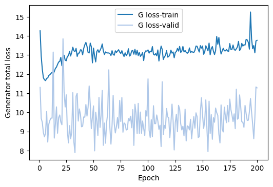
After the training is complete, we no longer need the discriminator and only keep the generator part of the network in order to produce new images. The disctriminator can be thought of as a loss function that is learned directly from the data, instead of being manually specified by the user. This is in contrast to typical losses such as the Mean Absolute Error and the Binary Cross Entropy loss frequently employed in deep learning. In general, a GAN has converged when both the generator and discrimimator losses have both converged, each around a stable value. Visually, the loss curve of a GAN that has trained properly looks something like this:

loss curve

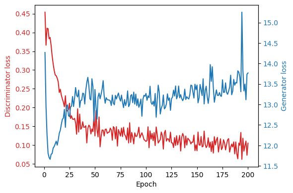
In the plot above we can see that the as the discriminator gets better, the loss of the generator increases as a result, until they both stabilize and the entire GAN has practically converged after 100 epochs or so. There is a small spike in generator loss at approximately 175 epochs but it returns to normal shortly after, so its probably nothing to worry about. While the above is an indication that the network as trained nicely, the only true way to validate this, is to evaluate it by translating and plotting some images of the test set. As with any deep learning model, the performance of pix2pix on the test set, is going to be worse that its performance on the training dataset.

Results¶

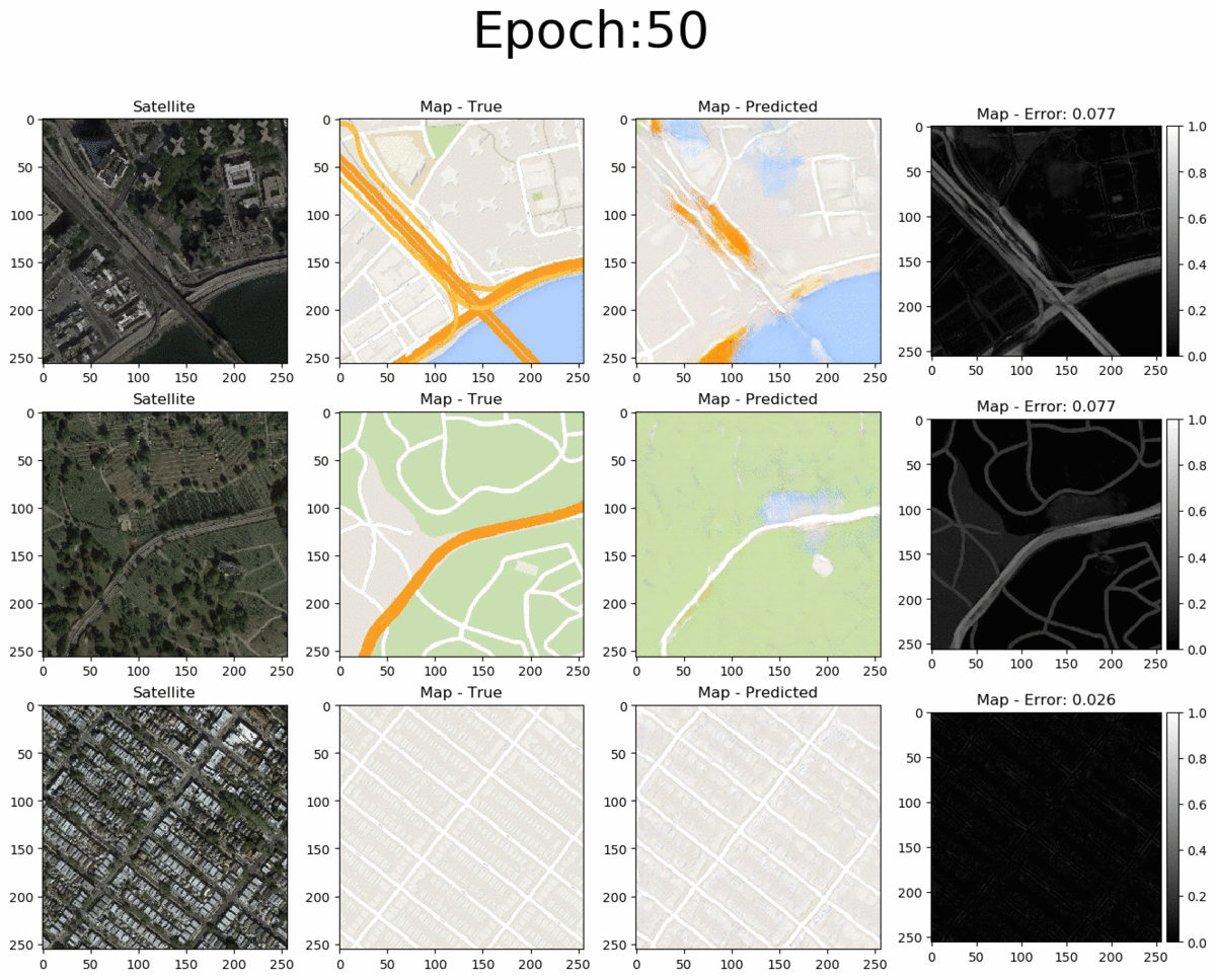
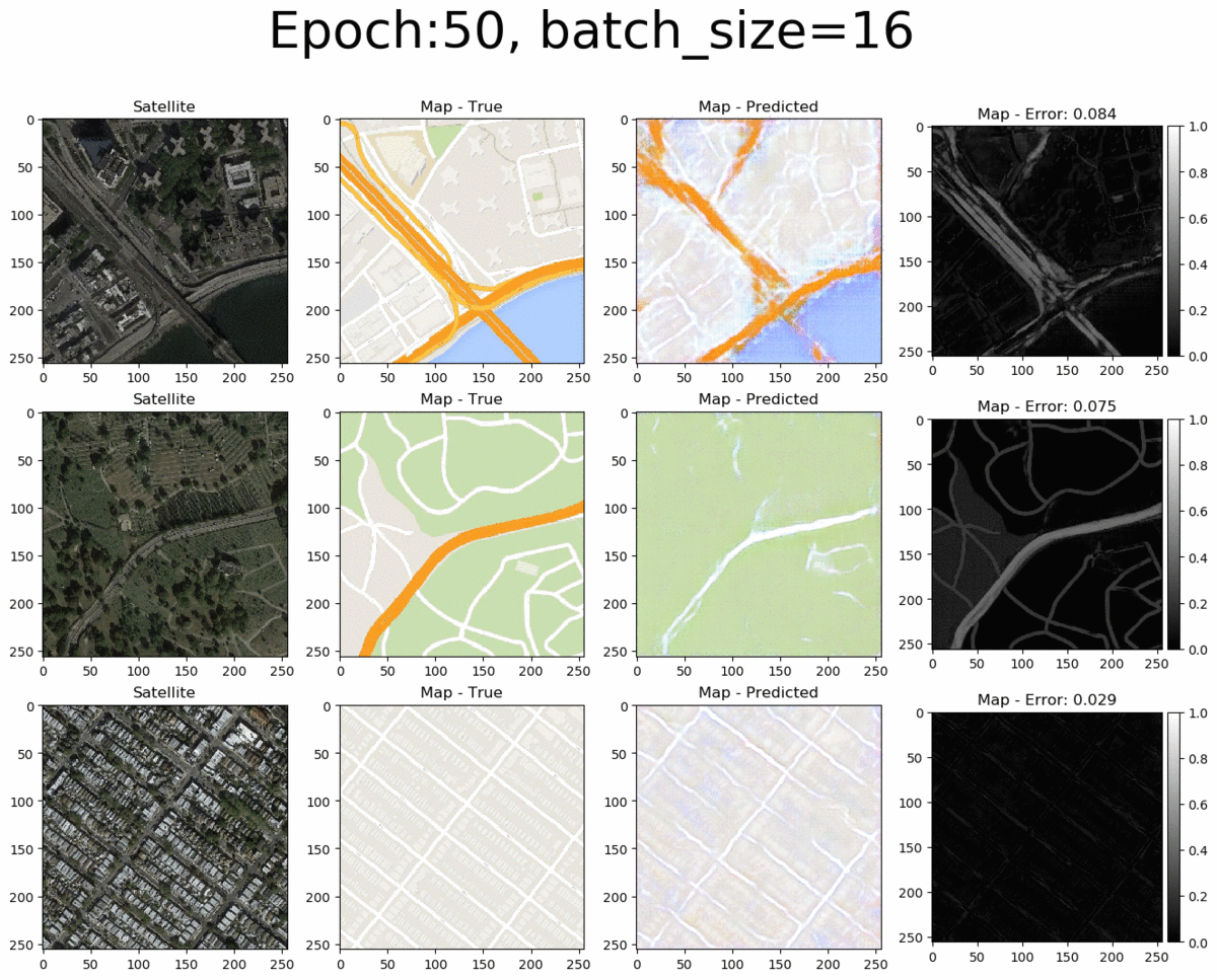
As we mentioned above, the most reliable way to evaluate the performance of a GAN is to manually inspect the quality of the generated images, preferably on a test set if possible. By examining the learning curve we expect that the model will converge after approximately 100 epochs and the results will be more or less stable after that. The baseline model below corresponds to the same number of parameters as the model in the pix2pix paper and is trained using a batch size of 1. Next, we can manually examine the quality of translated images belonging to the test set:

training gif

From left to right we see the input satellite image, it's true corresponding map, the pix2pix-predicted map and the error between the predicted and true maps (pixel-wise absolute error). The total pixel-wise error of an image isn't an accurate representation of image quality (as mentioned in the pi2pix paper). Nonetheless, manual inspection of the entire error map images allows us to easily detect where the model succeeds and where it fails. Overall, the pix2pix model is good at predicting the map for city blocks, as well as large green areas and bodies of water. However, it is not as successfull at fully coloring highways in orange. Interestingly, at 200 epochs, the model also draws what seems to be directionality arrows on the one-way streets of the bottom-row image.

The validation loss is not helpful in GANs¶

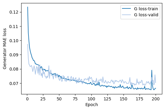As we saw from the training loss and after manual inspection of the generated images, the trained pix2pix model converges after about 100 epochs and the results of the model for 100, 150 and 200 epochs are quite close. However, if we look at the generator's loss on the validation set, we would get another picture. In the case of pix2pix, the generator loss has two components: (i) pixel-wise MAE and (ii) the discriminator's loss with respect to the generated image. The total loss of the generator is a weighted sum of these two components. valid loss curve MAE

According to the MAE loss on the validation set, the model overfits after 100 epochs, while we saw that is not the case. In general, if we were to believe the MAE loss of the validation set we could potentially cut of the training too early. valid loss curve total

If we look at the total loss, then the validation set is even less helpful, since it just seemingly randomly fluctuates from the beginning to the end of the training process around its mean value of 9.66.

The batch size can play a significant role¶

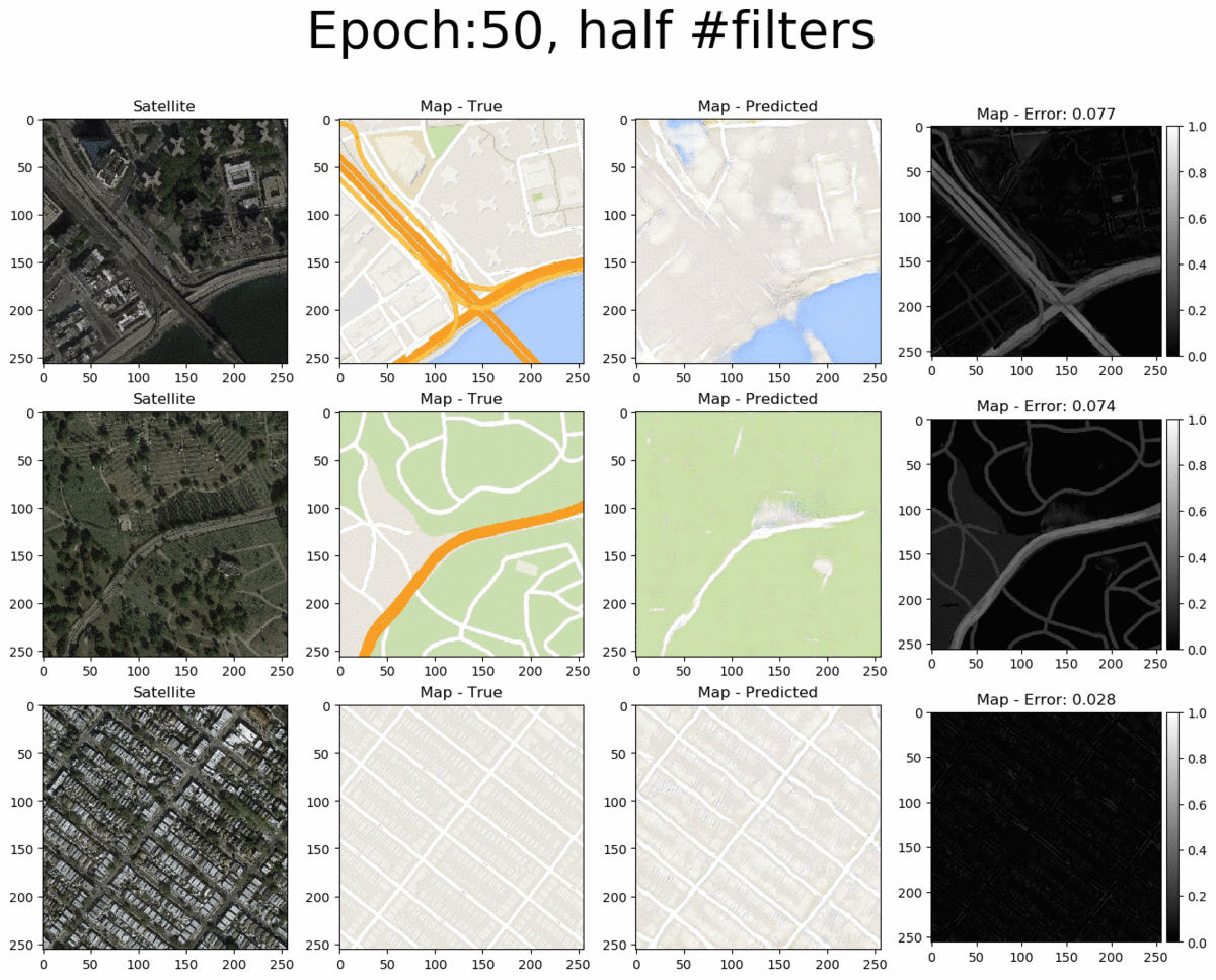
In the original pix2pix paper the authors suggest a batch size of 1 with the standard architecture of pix2pix (U-NET encoder) that we also implement here. If we change the batch size to 16, the quality of the generated images is worse, as demonstrated below: training gif batch size 16

Changing the model size does not have the expected effect¶

Typically, we expect a smaller model to be more regularized (or underfit) and a larger model to have more learning capacity (or overfit) depending on the task at hand and the number of available datapoints (in this case images). Below we perform two experiments: First, we train a model where all convolutional layers have exactly half the filter size, as well as a model where all convolutional layers have exactly double the numuber of filters. The models are called half and double "params" for simplicity, but it should be noted that this is not technically correct since halving or doubling the number of filters does not precicely halve or double the number of model parameters. As expected, the smaller model does indeed underfit the data compared to the baseline. Additionally, there's a training mishap a bit before reaching 200 epochs, but I still left the figure in to provide an example of what types of images can be produced from a model saved during a "bad" epoch. training gif half params

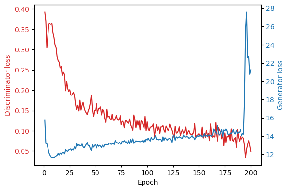
If we examine the loss curves below, we can see that something went wrong during the training process at the 196th epoch and the model did not return to normal by the last (200th) epoch. As such, it is more appropriate to use an earlier saved instance (e.g. at 150 epochs). training gif half params loss

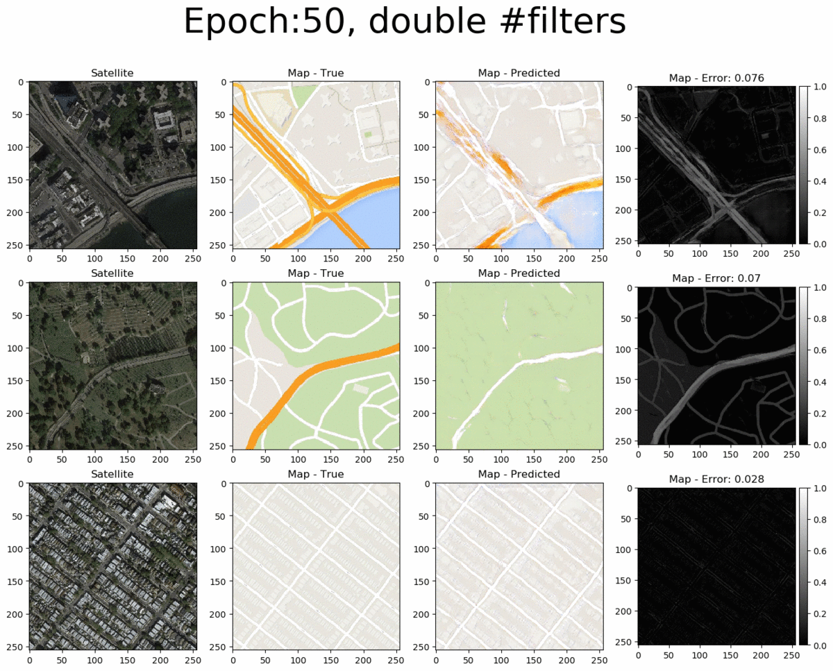
Next, let's look at the larger model. Counterintuitively, doubling the number of filters in the model does not significantly change the quality of the produced images. It does however significantly increase training time per epoch (as expected). Thus, there's no reason to opt for the larger model compared to the baseline. training gif double params

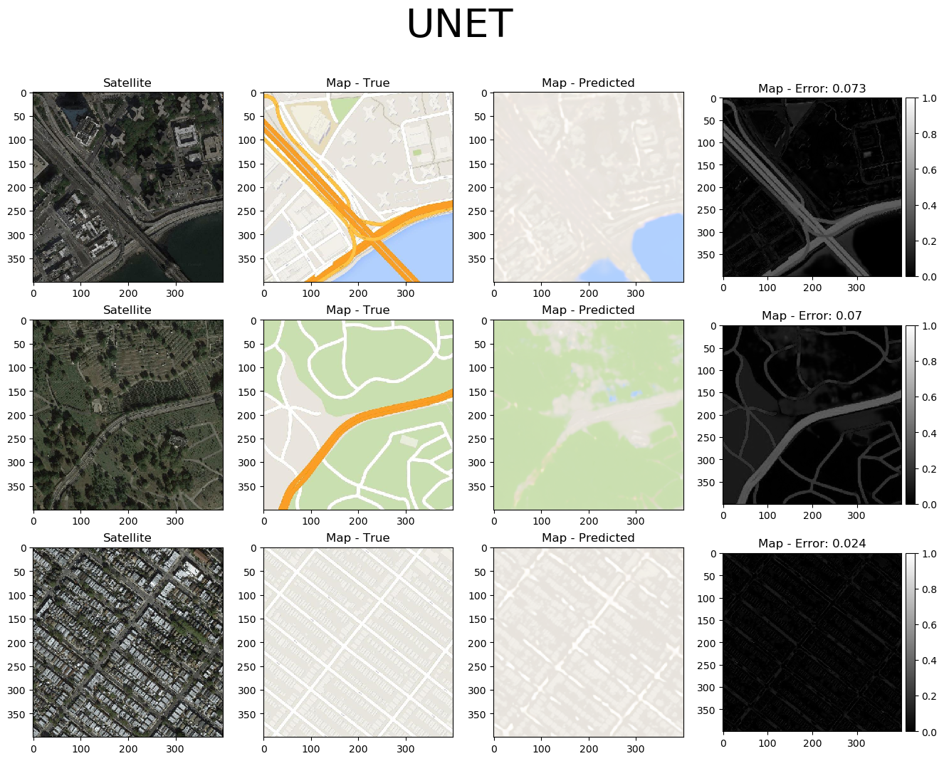
Why employing a simple UNET is not enough¶

Since we are already familiar with the UNET architecture used to generate an output image given another image as an input, we might be tempted to simply use a UNET for the task above, as well. The problem is that there (currently) is no way to accurately perform image-to-image translation with a fixed loss function, such as MAE. This is the reason we use the discriminator part of the network as a loss function that is learned directly from the data. As we can see below, when we employ a UNET with MAE loss to predict the map given a satellite image, the generated map images are not nearly as visually pleasing as those generated by the pix2pix GAN:

unet map

Additional Resources¶

Code availability¶

The source code of this project is freely available on github.